Self-Aligned ForcingStreaming Video Diffusion with Differentiable Noisy History

TL;DR

Five-minute explainer · narration with English subtitles

01 Overview

History stage and gradient flow

Autoregressive video diffusion reads the K/V of earlier blocks as history. Self-Forcing and HiAR detach it; SGF restores gradients through clean history using an extra rollout and replay. SAF instead uses differentiable noisy history from the same forward pass.

Paper Figure 1: Self-Forcing, HiAR, SGF, and SAF history stages, gradient paths, and forward-pass structure — The history stage and gradient path determine whether future losses can improve how earlier blocks encode K/V.

Why noisy history needs gradients

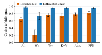
With a fixed LongLive checkpoint, noisier history can increase motion at the cost of imaging quality. With all other settings held fixed, restoring gradients through history K/V raises alignment with a matched bidirectional reference from 0.643 to 0.972.

Paper Figure 2a: history noise changes imaging quality and dynamic degree — **History noise changes quality and motion.** Only the history noise level varies; scores are normalized to imaging quality at t_c=0 and dynamic degree at t_c=750.

Paper Figure 2b: differentiable history increases gradient alignment — **History gradients improve alignment.** Only the K/V gradient path changes; error bars span multiple samples.

Aligned history, parallel rollout

At each stage, SAF gives the current block and its history the same noise level. One block-causal forward pass computes predictions and differentiable history together. Blocks roll out in parallel within a stage, while stages remain sequential; only a sampled exit stage retains gradients. A clean sink anchors appearance.

Paper Figure 3: block-parallel self-rollout, stage-aligned differentiable history, clean sink, and streaming inference — At inference, SAF^M reuses denoising K/V in one bank per stage for four-GPU pipelining. SAF^S shares one bank on a single GPU. Both avoid per-block timestep-zero recaching.

Training efficiency

SAF has the lowest memory and runtime in both settings: 1.41× faster than SGF in Chunk-wise and 1.82× in Frame-wise.

1 × GB300Batch size 44 critic-only + 1 joint update

Training memory and runtime per five-step cycle. Lower is better.
Method	Chunk-wise · 3 latent frames / block		Frame-wise · 1 latent frame / block
Method	Peak memory GiB ↓	Time / 5 steps s ↓	Peak memory GiB ↓	Time / 5 steps s ↓
LongLive	173.63	158.32	174.21	232.64
SGF	187.45	186.73	187.45	249.21
SDF	160.85	184.33	171.30	245.87
SAF	155.18	132.78	164.79	137.04

One GB300, batch size 4; local attention spans 12 latent frames in Chunk-wise and 21 in Frame-wise.

Inference throughput

SAF^M reaches 49.1 FPS in Chunk-wise and 21.6 FPS in Frame-wise with four-GPU pipelining. SDF and SAF^S share the same single-bank throughput.

SAF measured on 1 or 4 H100 GPUs; baseline FPS follow their published reports.

Inference throughput in frames per second.
Method / inference mode	Chunk-wise		Frame-wise
Method / inference mode	1 GPU	4 GPUs	1 GPU	4 GPUs
LongLive	20.7	—	—	—
SGF	20.7	—	8.9	—
HiAR	11.2	30.0	—	—
SDF	22.9	—	9.07	—
SAF^S Single KV	22.9	—	9.07	—
SAF^M Multiple KV	22.8	49.1	9.08	21.6